If you are stuck with the measurement of the decision tree loss function in your algorithm, you are at the right place. Decision trees are a very simple but very powerful type of supervised machine learning algorithm that is used to categorize or make predictions based on how a previous set of questions or choices were answered. This model is a form of supervised learning where the data is trained and then tested on a separate set of data that contains the desired categorization. As suggested, they are used for categorization or Classification problems generally but can also be applied to Regression problems.
Taking a Decision Tree beyond its capability, one can opt to make a Random Forest model which can help you to select the best features of your dataset as well. Read more here: Random Forest-Based Feature Selection
Note: A Decision Tree may not always provide a clear-cut answer or decision to the data scientist but, it may present options so the team can make an informed decision on their own. The idea of machine learning carries here as decision trees imitate human thinking and so thereby making it easy to understand and interpret the results provided by the algorithm.
How does a decision tree work?
As the name suggests a decision tree works just like a tree with branches. In Decision Trees, The foundation of the tree or the base is the root node. Then from there flows a series of decision nodes that represent choices or decisions to be made. These choices or decision nodes are called leaf nodes which represent the result of the decisions. The decision node represents a split point, and leaf nodes that stem from a decision node represent the possible answers. Just like leaves grow on the branches, similarly, the leaf nodes grow out of the decision nodes on the branch of a Decision Tree. Every second section of a Decision Tree is therefore called a “branch.” An example of this is when the question is, “Are you a diabetic?” and the leaf nodes can be ‘yes’ or ‘no’.
Find out more about Decision Trees here: Decision Trees
Did you know?
For errorless data, you can always construct a decision tree that correctly labels every element of the training set, but it may be exponential in size.
Some key terminologies
- A Root node is at the base of the decision tree.
- The process of dividing a node into sub-nodes is called Splitting.
- When a sub-node is further split into additional sub-nodes it is called a Decision node.
- When a sub-node depicts the possible outcomes and cannot be further split it is a Leaf nod.
- The process by which sub-nodes of a decision tree are removed is called Pruning.
- The subsection of the decision tree consisting of multiple nodes is called Branches.
What are loss functions?
A loss function, in simple terms, quantifies the losses generated by the errors that we commit when we try to estimate the parameters of a statistical model or when we use a predictive model, such as a Decision Tree, to predict a variable. Minimization of this expected loss which is called statistical risk is one of the guiding principles in statistical modeling. Undeniably, the ultimate goal of all algorithms of machine learning is to decrease this loss and any statistical risk it can lead to. The loss has to be calculated before we try to decrease it using different optimizers. A loss function can also be termed the Cost function. Since the calculation of the predicted variables is different for both the type of models in machine learning – regression, and classification, the loss functions of both are different.
Understanding Splitting Criteria or Impurity in the Decision Tree Loss Function:
It is common for the split at each level to be a two-way split. Although there are methods that split more than two ways, care should be taken when using these methods because making too many splits early in the construction of the tree may result in missing interesting relationships that become exposed as tree construction continues.
The scoring of the loss function in a Decision tree works on the concept of Purity in the split.
primary methods for calculating any existent impurity: Gini, and entropy.
Let us assume that for calculating the entropy, a set of 10 observations with two possible response values is used. For each scenario, an impurity score is calculated. Cleaner splits result in lower scores.
The formula for entropy is :

Entropy calculation is conducted on a set of observations as given which is S. The ‘pi’ here refers to the fraction of the observations that belong to a particular value and the ‘c’ given in the formula is the number of different possible values of the response variable. For example, for a set of 100 observations where the color response variable had 60 observations with “red” values and 40 with “blue” values, the p-red would be 0.6 and the p-blue would be 0.4. When pi = 0, then the value of entropy for this becomes zero.
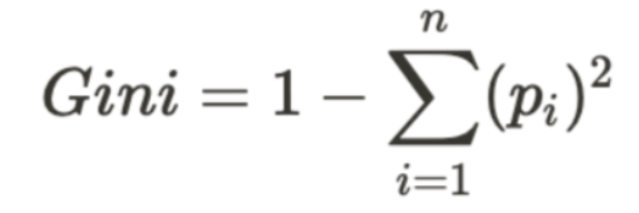
While entropy is the most preferred impurity measure, another similar method would be to use ‘Gini’ Impurity which is as follows;

The Gini impurity can be calculated by subtracting the sum of the squared probabilities of each given class from 1. As can be noticed from the formula, Gini Impurity can be biased towards bigger partitions (distributions) and easy to implement, whereas information gains can be biased to smaller partitions (distributions) with multiple values. Gini Impurity tells us if there is “success” or “failure” and can only split dichotomous variables and the information gained can evaluate the difference in entropy before and after splitting and illustrates existent impurity in class variables.
Find out more about the metrics here: How to calculate Gini and Entropy ?
You can use these as ‘criterion’ using the Decision Tree Classifier which comes with the tree class codes from the machine learning library ‘Scikit Learn’ that can be used to make a tree model using Python.

Find the copy-able code here:
from sklearn.tree import DecisionTreeClassifier
clf = DecisionTreeClassifier(random_state=0, criterion= 'gini')
clf2 = DecisionTreeClassifier(random_state=0, criterion= 'entropy')
Conclusion
From the aforementioned, we can observe that a decision tree is a bureaucratic approach to classification problems and regression problems alike. The use of values can be done to split the questions at each choice or branch and can end up in multiple leaf nodes which can be singular or dichotomous or multivariate. A small tree can be made easily but with a relatively high variance whereas a tall tree with too many splits generates better classifications but it probably is overfitting. So it is important to ensure that the right criterion or loss function is used and minimized in order to ensure that the tree is not overfitted or underfit. The Entropy or Gini metrics will prove helpful in this and can be instated at the beginning of the tree to split the branches accordingly. If you think one decision tree cannot take your model to take the right level of accuracy and performance it needs, then you can take the use of multiple decision trees which is called a random forest (another significant machine learning algorithm used by many).
To know more about Random Forests: Decision Tree vs Random Forests

An eternal learner, I believe Data is the panacea to the world's problems. I enjoy Data Science and all things related to data. Let's unravel this mystery about what Data Science really is, together. With over 33 certifications, I enjoy writing about Data Science to make it simpler for everyone to understand. Happy reading and do connect with me on my LinkedIn to know more!
- Yash Gupta
- Yash Gupta
- Yash Gupta


