The goal of this article is to help beginners understand the complex concepts of Deep Learning aka Neural network. I have tried to cover all the important concepts of deep learning a beginner would require, also I want to clarify that this article is for a beginner so I have tried to keep it as simple as possible, which means I am not covering mathematical parts here and tried to avoid few complicated terms. But in case you want to understand each topic deeply then I will link with some external sources, also for each topic I am planning to create a detailed article separately, so stay tuned with us.
What is deep learning?
Deep learning is a subfield of machine learning, which helps AI to understand our complex world in the same way, a human does. The way it works is inspired by the human brain(Neural networks). It is created with the goal of replicating human intelligence to build a smart machine(Artificial intelligence) that can automate our day-to-day job and a machine that can help us with complex problems like drug discovery, space exploration, etc. Deep learning is not a future tech, it’s already with us, helping us in answering our tons of daily questions(Alexa, Siri), treating complex disease (cancer, tumor), dropping us to our destination safely without any driver(self-driving cars), and in many more ways.
Why we need it
In today’s era where we generate huge amounts of data every single second need to be processed to extract meaningful insight. This data is so huge that it wasn’t possible to handle it with our previous method “Machine learning”. Machine learning requires features of data to be extracted manually, which is not possible with such huge data. Also even after doing that Machine learning performance’s stuck at some level, irrespective of the amount of data, which is another limitation. Also, Machine learning is not capable of handling complex data(real-world data). And deep learning handles this all problem very efficiently, without human intervention, it extracts the best features out of the data automatically, its performance increases with the increase in the amount of data also it handles complex data very well too.
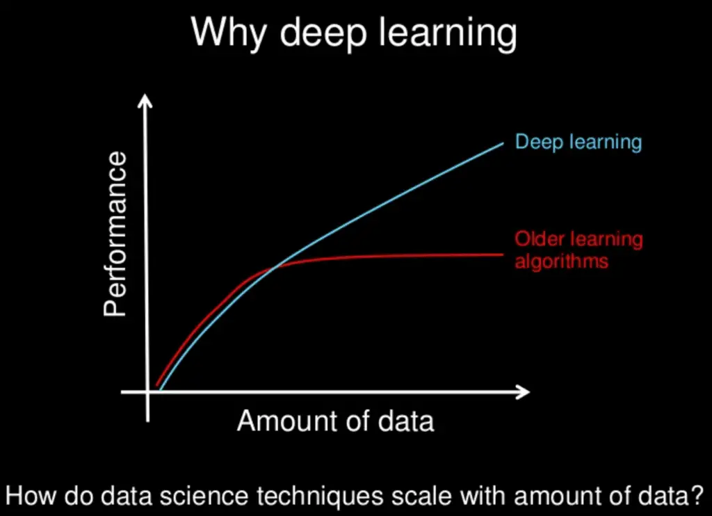
It doesn’t conclude that ML is complete garbage, it still holds its place in many situations like we always don’t have huge data or computation power to train a model and with less amount of data, machine learning performs better than deep learning most of the time (not always). So, they are like buddies, each one performs better in different use cases and will not replace each other, at least not in near future.
How Deep Learning Learns/works?
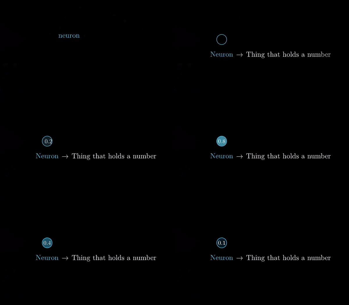
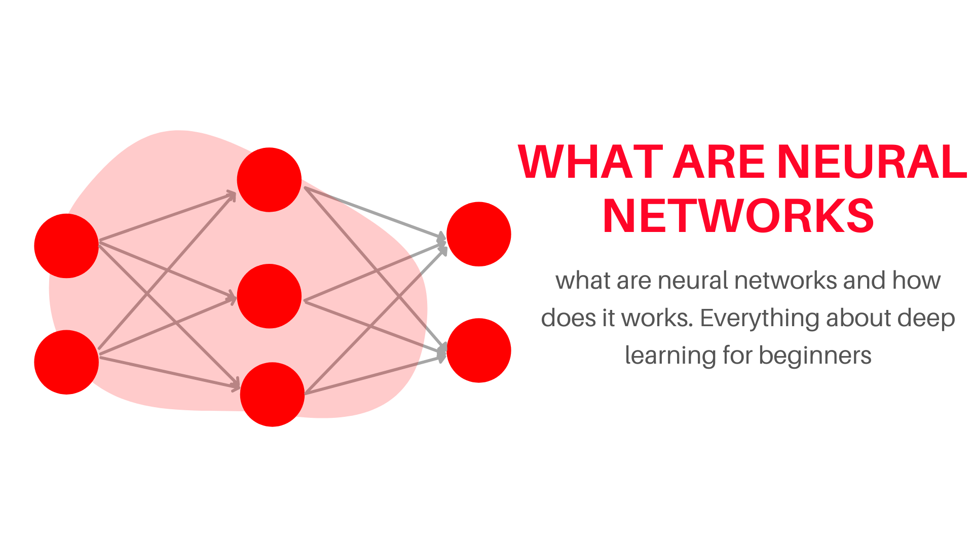
As we discussed earlier deep learning is designed with the inspiration of how the human’s neural network (brain) works. So, deep learning also has a neural network, called “Artificial neural network” also known as ANN through which it learns anything. Just like a human’s neural network, ANN is also built of lots of neurons that are connected to each other (how? We will discuss later), these neurons are the building block of a neural network. And all the information throughout the neural networks flows through neurons, if you are wondering what these neurons actually hold, the answer is very simple these neurons hold just a single number it could be anything integer or float, see fig1.0. We are currently looking at the neural network at its smallest level, so if you zoom out a little bit, you will be able to see lots of layers connected to each, which are of course made of those neurons. These layers can be separated into three different parts, i) Input layer ii) Output layer iii) Hidden layer. So let’s briefly look at these
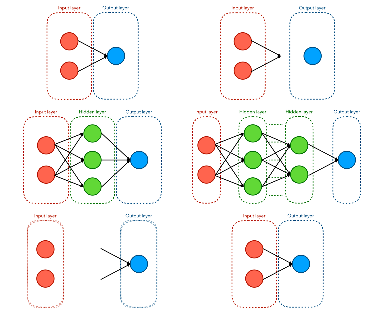
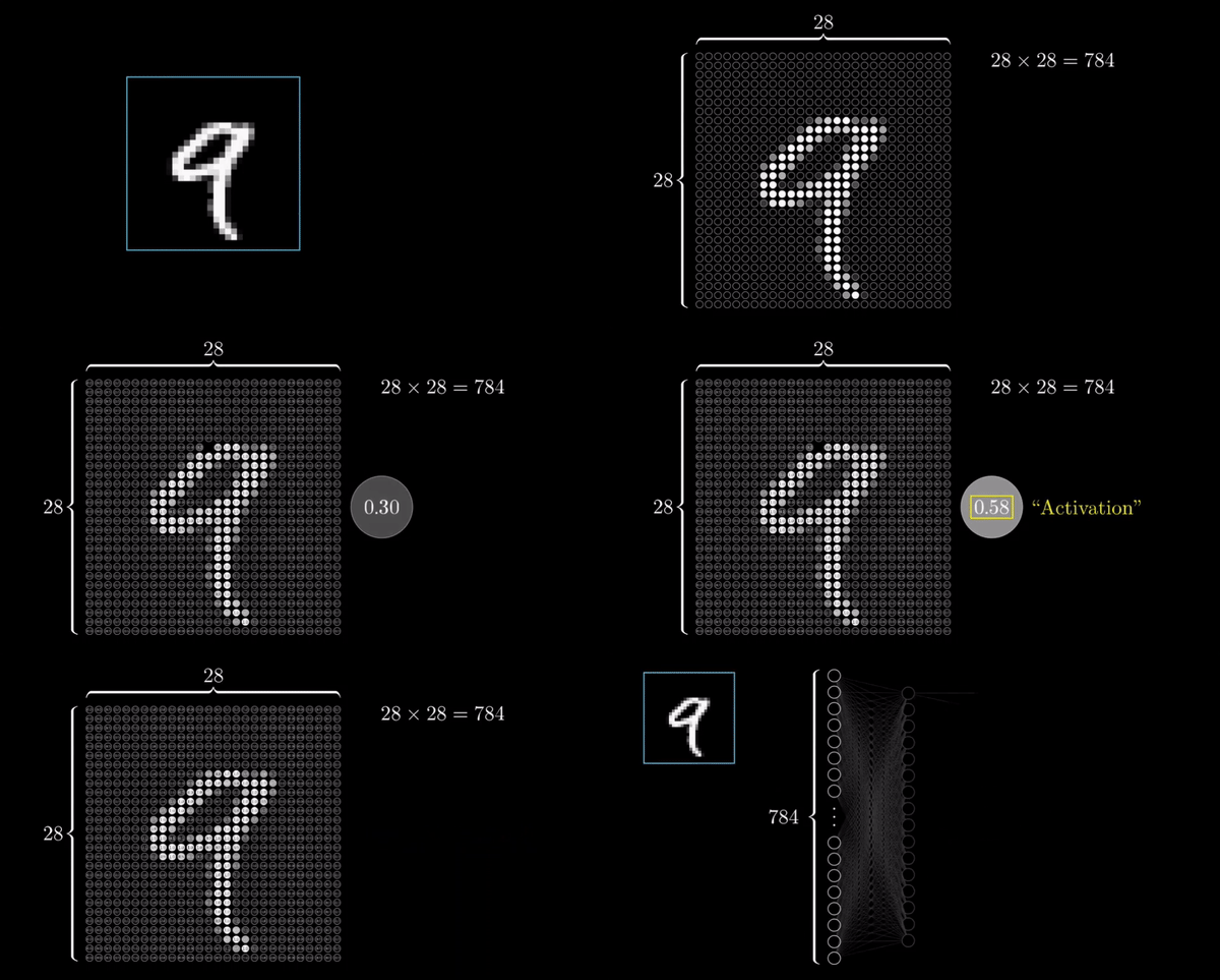
i) Input layer– It is always the first layer of any neural network, it takes all your data as input. These inputs are stored in a neuron and the number of neurons in the input layers depends on the size of data, for example, a black and white image of size 28×28 will have 784 pixels, so this will be the number of inputs of your model, which is equal to the number of neuron of your input layer, and these neurons will hold the number(color scale) ranging from 0 to 255(Generally we convert these value on the scale of 0 to 1) depending on the color/light intensity for example if the particular pixel is black then the neuron taking that input will store value as 0 or if the color is white then that neuron will store the value of 255( or will store 1, if you have scaled your value) and the number in between 0-255 depicts different shades of gray. So this was just for black and white images, what if you have a colored image, then its input will be something like this 28x28x3, where 3 represents different color channels(Red, Green, and Blue) and 28×28 is, of course, it’s size. So if you will calculate 28x28x3 it is equal to 2352, which is literally a huge amount of inputs/neurons in the input layer, just imagine it. Okay so this was your input layer now, let’s move further to the output layer
ii) Output layer– This layer is always the last layer of your neural networks. It outputs the class/value of the data for example let’s say you have created a model to classify a cat or dog. Then your last layer will output the probability of different classes your test image likely can fall to, for eg suppose you have passed a dog image to test, then it will output something like Dog-0.98 and Cat-0.02.
iii) Hidden layer– It is where the actual magic happens this layer is also known as the black box. This is the most important layer of any neural network because this is where your model actually learns. This layer can have multiple or no layers, a neural network with 0 hidden layers is known as a perceptron, it has only an input and output layer, on the other hand, a neural network can have millions of layers. The more hidden layer a neural network has the complex it will get, resulting in a better model performance at the cost of high computation power and time because it can take you months to train. The number of hidden layers and the no of neurons in a hidden layer is decided by a trainer.
So, this was all about layers of the neural networks. Alright, now you know that deep learning learns through a complex neural network formed of lots of layers and which is further formed of lots of neurons. Now you might have questions about how these neurons and layers are connected to each other and how the information flows in a neural network. So, let’s explore it.
Data propagation in Neural network
I am going to introduce you to some new terms, which are important and may confuse you but, don’t worry I will discuss that later in this article. So, take a deep breath and dive in
Also read- How to toonify yourself -with code
Forward Propagation
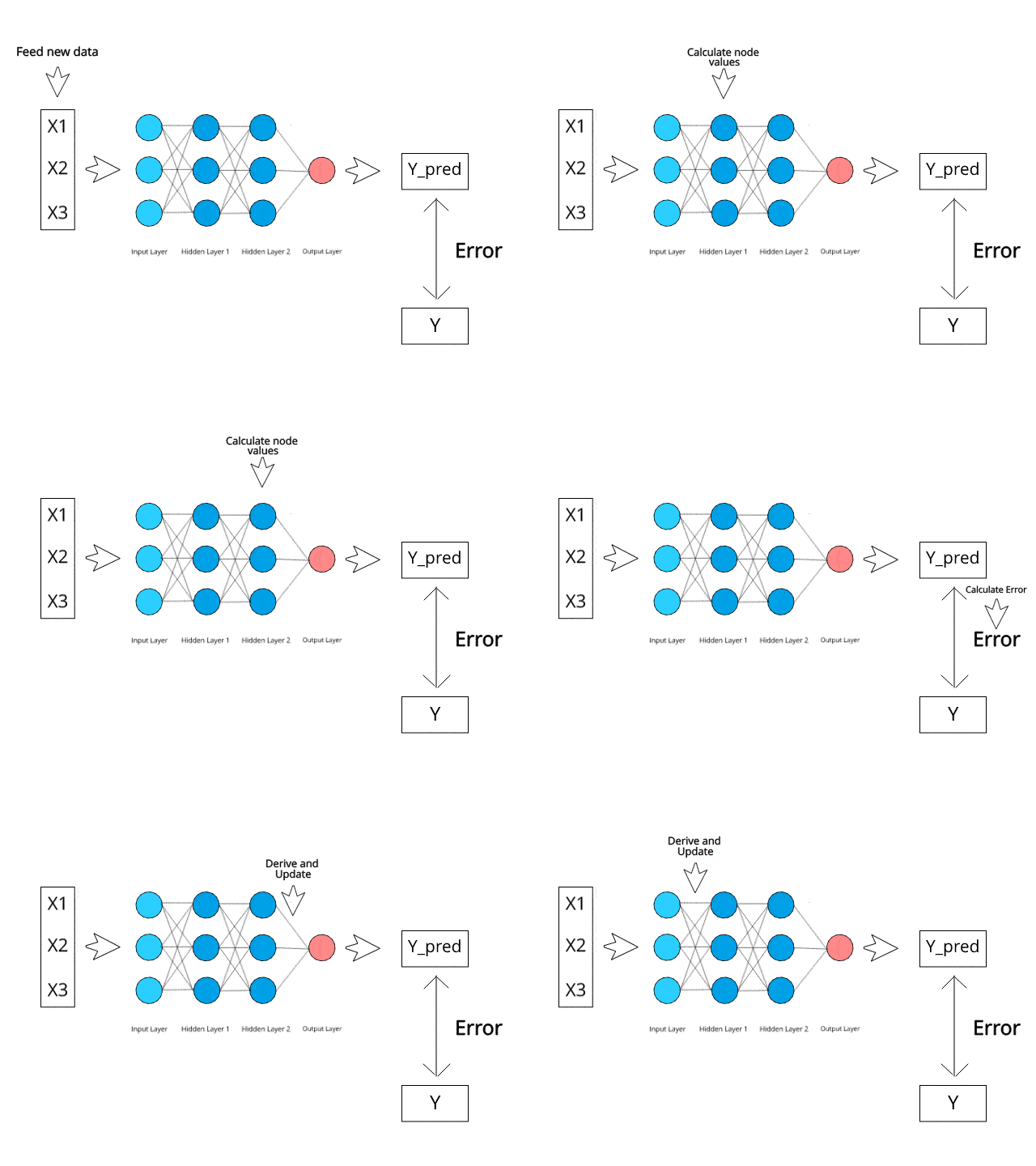
The information flows from the input to the output layer, the neurons X1 to Xn of input layers connected to the next layer (hidden layer) through channels which are assigned to a random numerical value called weights (weights tells a neural network how important a particular neuron is). The inputs are multiplied to the weights and their sum is then sent as input to the next layer, where each neuron, in turn, is associated with a numerical value called bias which is then added to the input sum. This weighted sum is then passed through a nonlinear function called activation function (which decides if that particular neuron can contribute to the next layer or not). And finally, it passes to a final layer (output layer) which returns a probability value (the neuron with the highest probability value is the final output). This type of data flow where information is moving forward as its name called forward propagation.
Back Propagation
The back propagation is reverse of the forward propagation, like in forward propagation data propagate from input to the output layer, here in back propagation the data propagate from output layer to the hidden layer(not to the input layer) to fine-tune the weight which was originally random value. Back propagation is the main reason why neural networks can learn by themselves. Let’s see how back propagation happens and how it improves our model.
So, after the data is passed to a final layer and we get a prediction, we compare it with the original output that it’s true or not (most of the time output will be wrong in first forward propagation), if the prediction is correct we leave it or else we pass it to a loss function which calculates how deviated the prediction is from the expected output which is then passed to an optimizer function that updates the weight of each neuron to fine-tune the output.
Components of Neural network
Okay, so now we know how data flows throughout the neural networks and how it learns and improves itself. I know those technical terms are scratching your head, so let’s take a look at those as well.
Weights
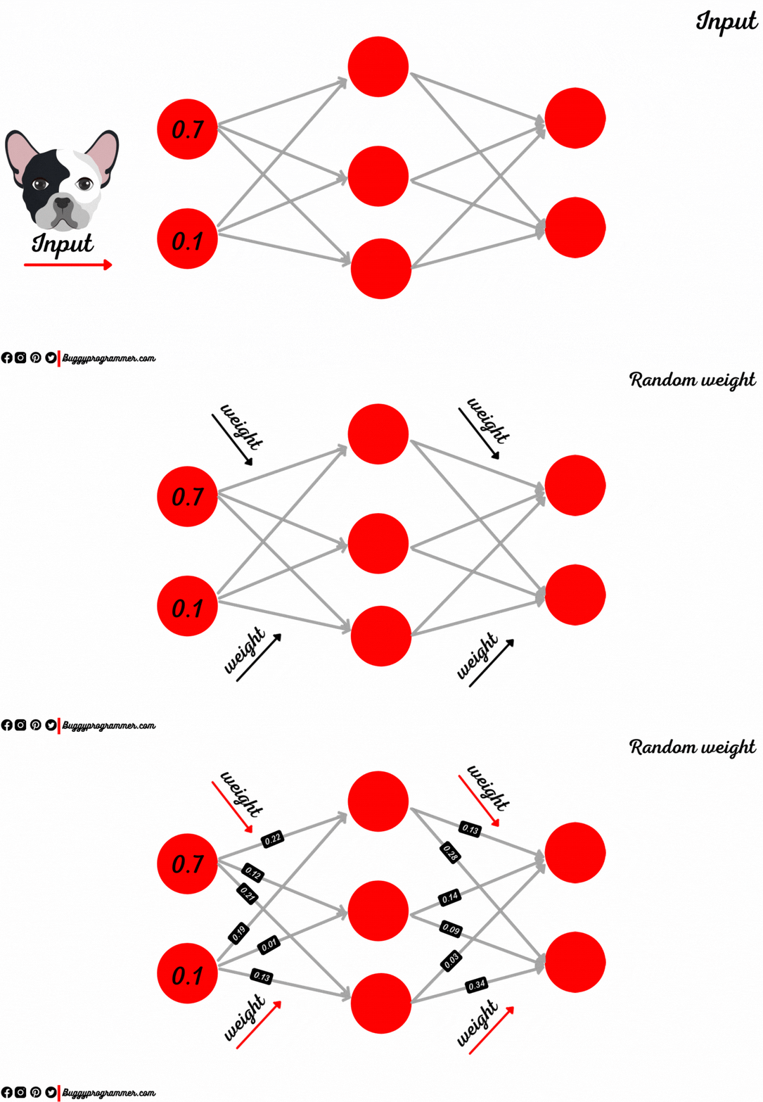
Weights are numerical values assigned to each neuron to connect two neurons, and it tells the neural networks how important a particular neuron is for the training, depending on its value. At first forward propagation, the weights of each neuron are literally assigned with a random value, then it is fine-tuned with each epoch to find the best weight
Activation Function
After receiving a weighted sum as input from the previous layer (input layer or hidden layer before current layer) it decides whether a neuron should be activated or not. The main purpose of the activation function is to introduce non-linearity into the output of a neuron the reason is that without a nonlinear function in a neural network, no matter how many layers you add, it will behave like just a single layer perceptron, because if you add all those layers you will get another linear function. So, it is important to have a non-linear function (activation) that adds complexity to the model.
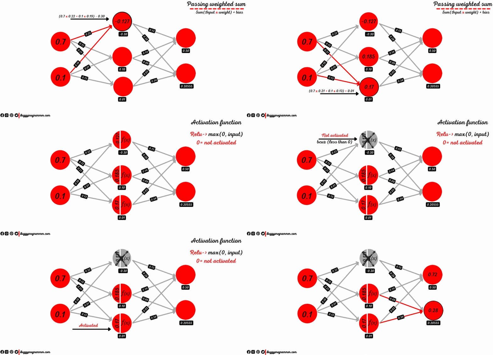
We have many activation functions in deep learning, which decide differently whether a neuron should activate or not. Some of the examples of activation function are
- Linear function
- Sigmoid
- Softmax
- Tanh
- Relu
Let’s understand this by an analogy, suppose you are a leader of a certain 10 boys/girl group (each person is a neuron) and you guys are trying to enter a big apartment, but you find out there’s a watchman (activation function) on the main entrance gate and can only let you in if you give some good reason or somehow if you can convince him that your friends or family live in there. So to find a reason you asked your all friends of your group to think of a good reason (each reason is a weight of the corresponding neuron), then you summed up those all reason of your friends and created a final reason (think of it as weighted sums =sum(all inputs multiplied with their corresponding weight). After all this you finally went to Watchman (activation function) and told him the reason why you want to enter the apartment now, he will decide whether your reason is enough to enter the apartment or not.
if you want to learn more about it you can visit here
Bias
Bias is like a threshold for a neuron and determines if a neuron should activate or not. It increases the flexibility of the model. You might have a question that we learned that activation function is the one which decides that a neuron should activate or not right! Yeah, you are right, actually what happens is activation function has a predefined threshold and a neuron will only activate when it crosses that threshold, but sometimes we require a different threshold which is not possible with activation function, so we add a bias in the weighted sum before passing it to the activation function.
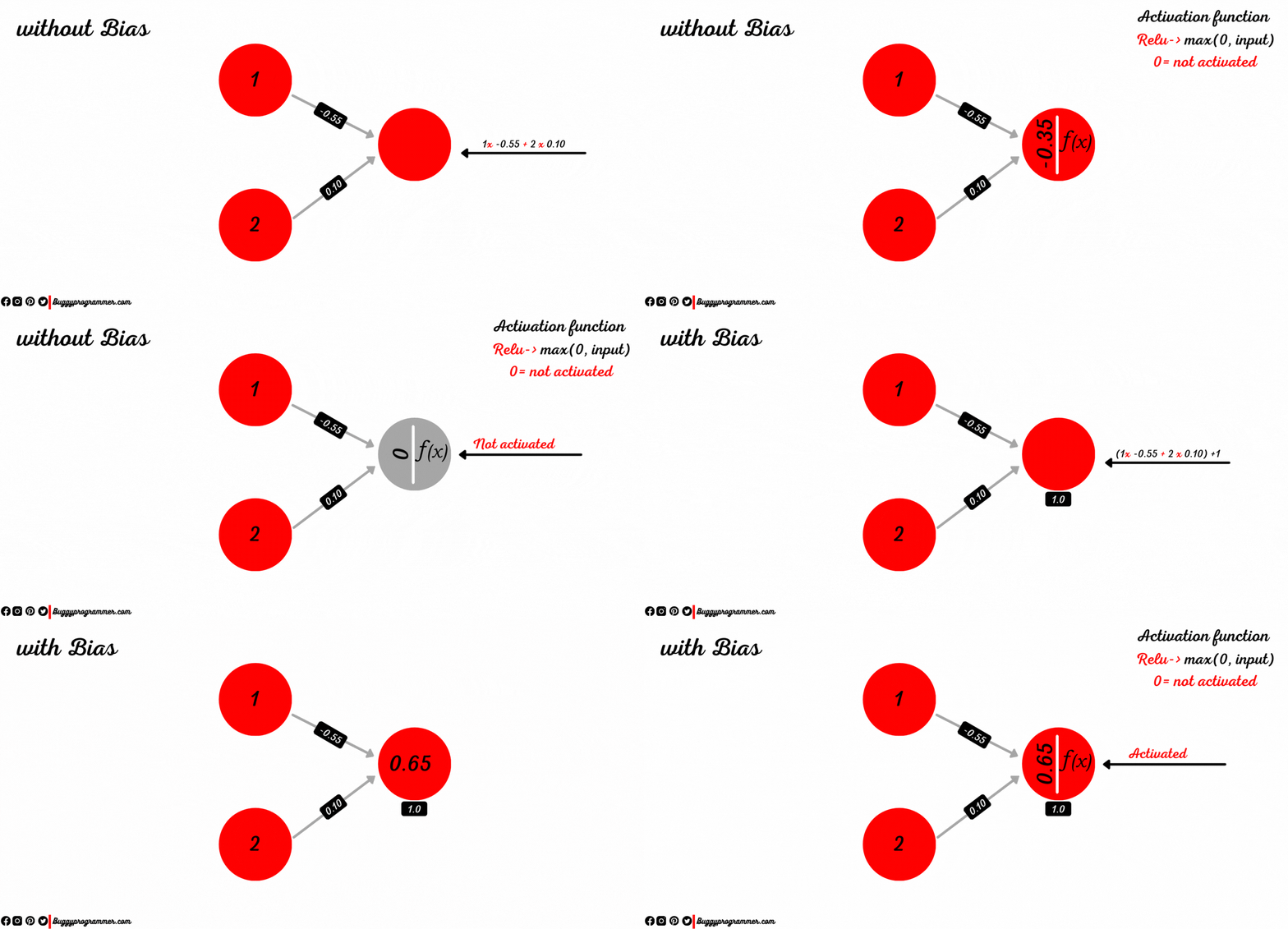
Let’s understand this with an example suppose you have a weighted sum which is equal to -0.35, so if you use “Relu” here as an activation function whose value is “max(0, your input)” means it will only activate if your weighted sum is greater than 0 so, in our case, it won’t activate. But what if you want to shift the threshold and want to activate it when your weighted sum is let’s say “-1 <=” (greater than or equal to -1) instead of “0 <” (weighted sum greater than 0). We can do that by using a bias in it, we add bias to the weighted sum before passing it to the activation function, so if you want to shift the threshold to “-1 <= ” from “0 <”, you can add “1” to the weighted sum. Like if you add 1 to -0.35 it is equal to 0.65 which is greater than 0 so it will activate.
Now you might have questions about why we added 1, we added 1 because we want to shift the threshold from 0 to -1 so for example if you want to shift the threshold to -5 we would have used 5. Basically, it is the opposite of the number you want to shift with. One more example would be if I want to shift it to 5 then use -5.
Bias is a learnable parameter just like the weight so it also changes after each epoch and also bias is not chosen or tuned by the programmer, it is done automatically.
Loss function
Now it’s the time to discuss loss function. The loss function is used to calculate the deviation of the predicted value from the actual value. It is calculated after every epoch and SGD(optimizer) constantly works on it to improve. The accuracy of any model is directly proportional to the error a model has, so it’s very important to minimize the error.
For example let’s say you passed a dog image to test your model which classifies dog and cat, returns the output as “Dog=0.46 and Cat=0.54” which means your model classified your image as cat (higher probability), which is wrong. Now as we discussed earlier that when your model gives a wrong prediction we pass it to a loss function, which calculates the deviation of the predicted output from the expected output (Dog=1.0 and Cat=0.0), and this error is then passed to an optimizer which updates our weight
We have various loss functions out there, which we use in different cases and scenario . Few of them are
- Regression: Squared Error, Huber loss
- Binary Classification: Binary cross-entropy, Hinge loss
- Multiclass Classification: Multiclass cross-entropy, Kullback Divergence
Optimizer
During the training, we fine-tune the different parameters(weight, bias) of the model to minimize the loss function of the model to make our model as optimized as possible. To optimize our model, optimizers rely on the help of loss function which guides it on the process of fine-tuning weight and bias. Loss function helps the optimizer to know which weight and bias should be increased and which should be decreased. There are various optimizer which helps in model optimization differently, some of the examples of optimizer are
- Gradient Descent
- Stochastic Gradient Descent
- Adagrad
- Adam
- RMSprop
Learning rate: Learning rate is a hyperparameter that controls how much we are adjusting the weights with respect to loss. If we set it to the high value we might miss the least loss we could have ever got and if we set it to the low value, we could end up waiting for our whole life. So, it is important to choose the learning rate very carefully, it should not be too high nor it should be too low. Usually, we use a small learning rate like 0.001.
To understand it better, let’s suppose you are watching a movie on Netflix and unfortunately you missed your favorite scene and you don’t remember its time frame. So you decided to search it by going back and forth by 5 minutes (high learning rate), you noticed that you went through the whole movie at an interval of 5 minutes but you did not found the scene, so you now decided that you will reduce 5 minutes to 5 sec and give it a try again, but this time you noticed that it’s taking too much time.
Similarly, if you choose too high or too low a learning rate, it will be hard to find a model with the least loss score. If you are interested in learning more about learning rate, you can read here
Parameter vs Hyperparameter
The parameter which is often referred to as a model parameter is something that is internal to the neural networks and anticipated by the model itself on the basis of data. Parameters are not decided by the programmer or trainer, examples of parameters would be the weight and bias of the model. On the other hand, Hyperparameter is a configuration that is external to the model and whose value can not be anticipated from the data. The Value of the hyperparameter is decided by us to improve the model performance for example epoch size, batch size, learning rate, etc.
Epoch Batch size and iteration
Epoch: As we saw here how the data propagate in the neural network through forward propagation and how it improves itself through back propagation, so actually we have a term for this forward and back propagation called Epoch. One epoch is when an entire dataset completes a revolution of forward and backward through the neural network. The more epoch a neural network trained for, the better it gets but if you train it for too much epoch it will overfit your model which simply means that your model will memorize the data and will perform best in training data and worse in testing data.
Batch Size: Oftentimes we have a huge dataset and passing that huge dataset at once to the model can take you so much time and maybe not be able to process it, especially if you don’t have good computation power. So to deal with that problem we shuffle our whole dataset and then separate it into small chunks called batches and then we pass it to the model. We shuffle our dataset to make sure that our model get exposed to all kind of data of our dataset and not just get biased toward single type of data, this is very important step. So the number of records we choose in a single batch is known as batch size. For example, suppose you have a dataset with 100 records then you divide the dataset in small chunks(batch) of 10 records then your batch size would be 10.
Iteration: Iteration is nothing but the total number of batches you have after separating the dataset like in our above example we divided the 100 records dataset into batches of 10 records so 10×10 records = 100records which concludes that we have 10 iterations. Iteration can also be thought of as the total number of times you need, to pass your all data batches to the model, to pass a complete dataset.
I hope you learnt something from this 😀. If you have any question/suggestion pls feel free to use comment section.

Data Scientist with 3+ years of experience in building data-intensive applications in diverse industries. Proficient in predictive modeling, computer vision, natural language processing, data visualization etc. Aside from being a data scientist, I am also a blogger and photographer.
- Aman Kumar
- Aman Kumar
- Aman Kumar
- Aman Kumar
- Aman Kumar
- Aman Kumar
- Aman Kumar
- Aman Kumar
- Aman Kumar
- Aman Kumar
- Aman Kumar
- Aman Kumar
- Aman Kumar

