Is it important to know the assumptions of linear regression? How does it affect your model and what should you take care of, we will see all these in this blog.
It is very important that you first check the pre-requisites or assumptions of any model before implementing it because this gives you an idea of whether the model you are going to apply will give good results or not. So, today we are going to talk about such assumptions of the Linear Regression Model, and remember this, it is very much important from the interview point of view.
I have faced questions on this topic in the interview many times.
Let’s first understand what is Linear Regression. It is very simple to understand and implement too.
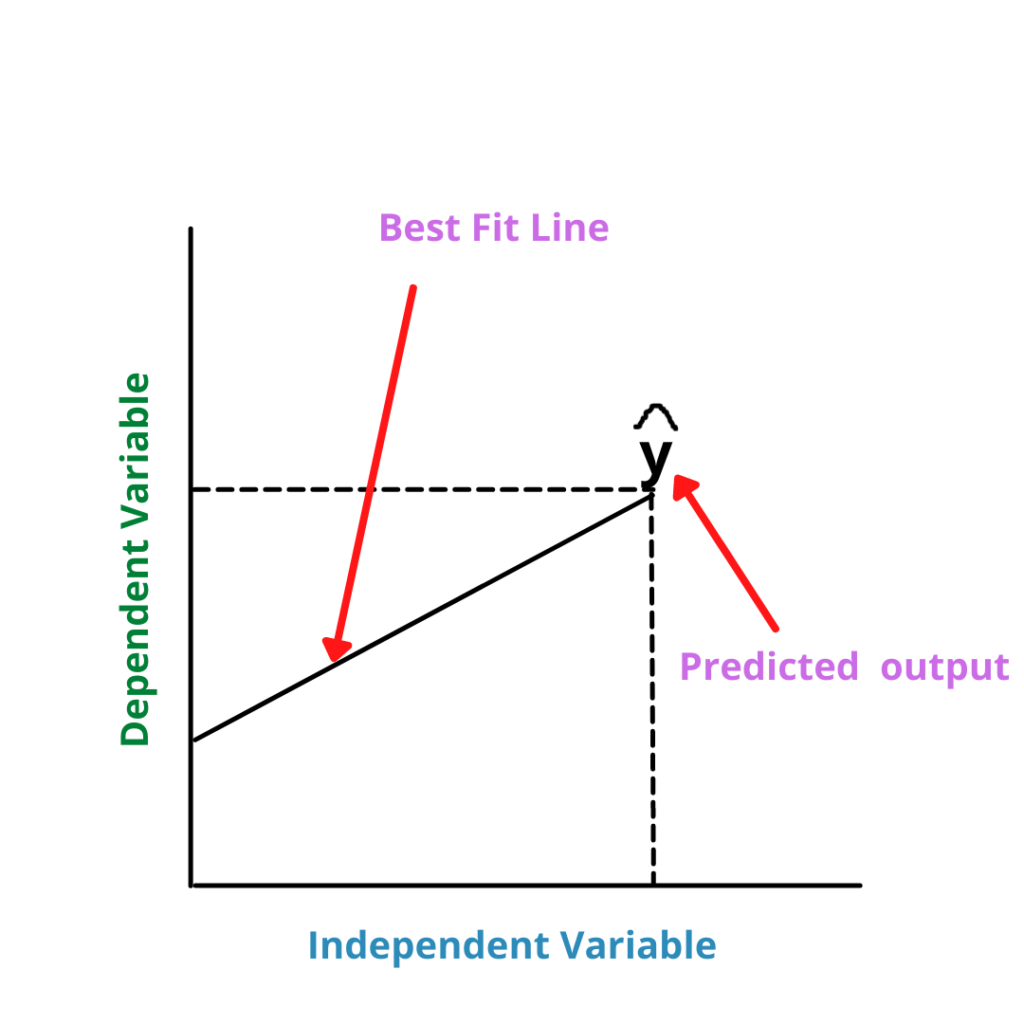
In Linear Regression we find a relationship between the Independent (X) and dependent (Y) variables and draw a straight line. This straight line is called as Best Fit Line. We analyze, on change in the independent variable, how it affects the dependent variable? Does it increases or decreases.
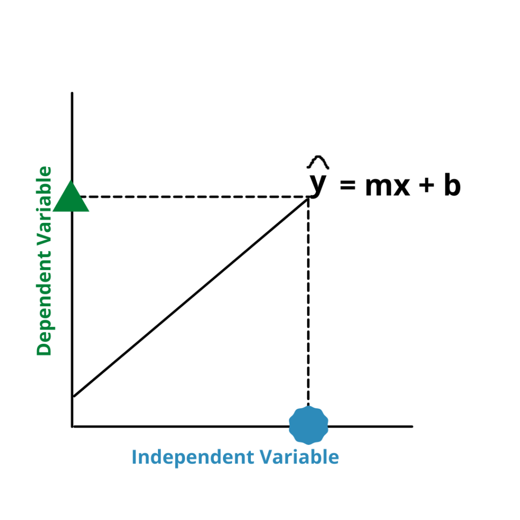
As the value of X increases, the value of Y also increases as well, this is called Positive Linear Regression as it has a positive correlation that is the reason there is + sign in the below formula,

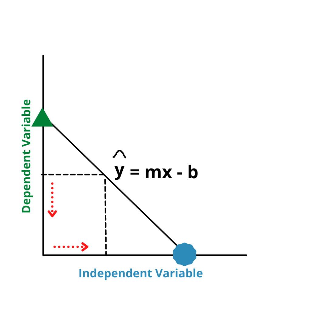
When the value of X decreases, the value of Y also decreases as well. This is called negative Linear Regression as it has a Negative Correlation
Let’s start with understanding the Assumptions of Linear Regression
- Linearity: Linear Relation between Dependent and Independent Variable
In Linear Regression, the first assumption of linear regression is that a straight line should be able to explain as good a relationship as possible. If it is unable to do so then the assumption of Linearity fails.
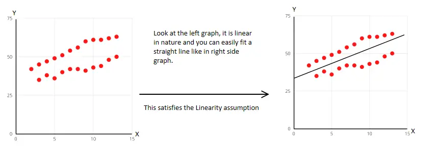
Look at the left graph, it is linear in nature and you can easily fit a straight line like in the right-side graph.
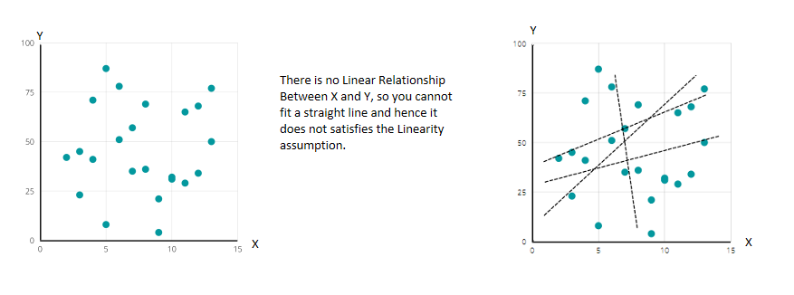
There is no Linear Relationship Between X and Y, so you cannot fit a straight line and hence it does not satisfy the Linearity assumption.
Also, read → What is Bias vs Variance trade-off?
2. Normal Distribution of Error
The second assumption of linear regression is that the Residual or the error distribution should be normally distributed. To calculate the error, use the below formula,

This is not a big issue if the normality of error is violated in the case of large data because, in the case of a large amount of data, the underlying relationship can come out.
What happens if there is a violation?
If the data is small then violating the normality of error can affect the standard error. The graphical way you can detect is via Histogram.
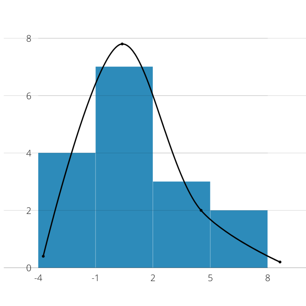
This is Histogram, you can see the line graph on the histogram which is almost Normally Distributed, which means that your data is not violating the Normal Distribution of Errors.
3. Homoscadasticity (no Heteroscedasticity)
The third assumption of linear regression is that errors should have constant variance or homoscedasticity. Let us just understand it visually.
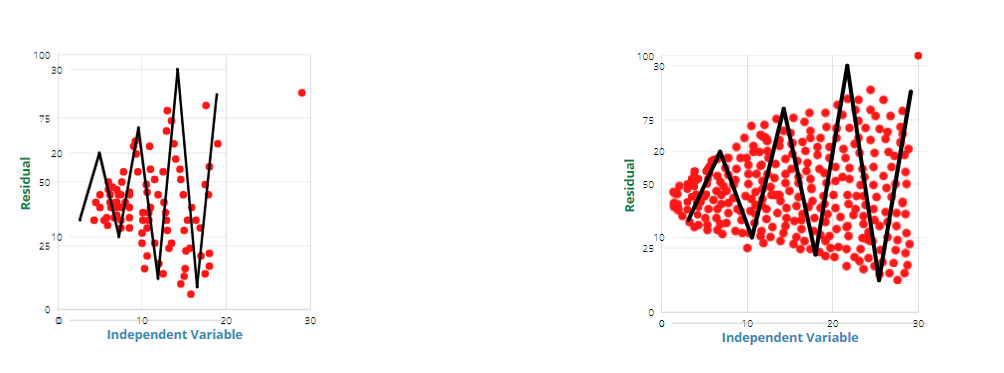
Looking at both these graphs, the variance in the residuals (Line chart) can be explained by the independent variable. When the independent variable(X) increases the variance in the error is also increasing, which means the error which needs to be constant is not at all constant in these two graphs. This is the case of heteroscedasticity, which means, it is violating the Homoscadasticity assumption.
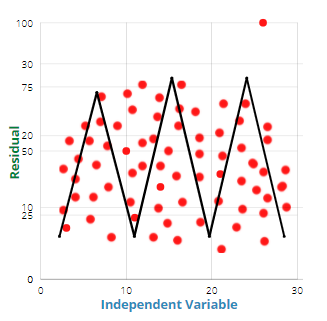
Now look at this graph on the left side, you can see that the error or residual is constant throughout every value of X. Now, this is the case of homoscedasticity and it satisfies the assumption.
To understand more about Homoscedasticity: What is Homoscedasticity?
Problem with Heteroscedasticity:
It affects the standard Error and hence the level of significance becomes unreliable. Because when the variance changes, the distribution of data also changes. For e.g. If there is Heteroscedasticity then it can result in Leptokurtic distribution instead of Platykurtic distribution or Normal Distribution
OR
Can result in Normal Distribution instead of Platykurtic distribution or Leptokurtic distribution
OR
Can result in Platykurtic distribution instead of Normal Distribution or Leptokurtic distribution
So this changes the significance of data i.e. p-value and we cannot rely on that.
Detection: You can detect Heteroscedasticity via
- Residual Plot (The graphs above are examples of the residual plot)
- Goldfeld Quandt test
- White’s Test
Treatment: Some ways to treat Heteroscedasticity is:
- Weighted Least Square
- via Logarithm
4. Multicollinearity:
The fourth assumption of linear regression is that when 2 or more independent features are correlating with each other then the problem of multicollinearity comes into the picture.
for e.g. Y = m1X1 + m2X2 + b
In Linear Regression, we analyze the change in Y when there is some change in X. So when X1 changes we measure the change in Y keeping other independent variables constant and the same with X2. But, what if when some change in X2 also affects X1 along with Y. This is Multicollinearity, change in one independent variable changes another one too.
Let’s take an example,
(House Price) = m1(area sq.ft) + m2(number of Bedrooms) + b
In this example, we have taken y as House Price, X1 as area sq. ft, and X2 as the number of Bedrooms. So, area and number of bedrooms are proportional to each other, as area increases, the number of bedrooms can also increase and both factors can increase the price of the house. I took this example specifically to explain Multicollinearity.
Now, when the area sq. ft changes there is some change in the price of the house, but a change in the area also affects the number of bedrooms in the house, which means both the independent variable have changed when only either independent variable was changed. So, you can’t really explain on change of which independent variable, the dependent variable i.e. House Price was increased or decreased.
| Area sq.ft | Number of bedrooms | Number of bathrooms | |
| Area sq.ft | 1.0 | 0.9 | 0.6 |
| Number of bedrooms | 0.9 | 1.0 | 0.4 |
| Number of bathrooms | 0.6 | 0.4 | 1.0 |
This is a correlation matrix of independent variables, The correlation between the Number of Bedrooms and Area sq. ft is 0.9 which means they both are highly correlated with each other and there is high Multicollinearity between them. Many resources say that correlation of 90% is very high and you should take action against it.
Problem with Multicollinearity:
You cannot rely upon the standard error, the variance in the coefficient will be inflated. By inflation in the variance what I mean is explained via the diagram below, look at the 1st figure, the data is accumulated closer to the mean of distribution but due to Multicollinearity, the variance has been increased which can be understood from figure 2.

Ways to Detect Multicollinearity:
- Correlation Matrix: This is shown in the above table. Python’s seaborn library can make this, use seaborn’s heatmap to plot this correlation matrix.
- VIF score: Variance Inflation Factor, gives a VIF score for every independent variable. If that score is above 10 then that variable is highly correlated to some other variables in the data and you need to take action for treating it. Using Python you can find out your VIF score very easily. The VIF formula is given below.

Treatment:
- You can combine the correlated features to get the new feature which can solve Multicollinearity, this is a part of feature engineering but this is possible only when you understand the data, i.e. you need to have domain knowledge of data.
- Don’t do anything, Remember that Multicollinearity does not affect prediction, so if your goal is prediction, leave multicollinear features as it is.
- Drop one of the correlated features, But what if the feature that you delete is the important feature, this means you cannot drop without finding if the feature is needed for the task or not. So you can follow the next step.
- Increase the sample size of your data.
We hope you understand Linear regression better now and also the assumptions of linear regression. For more such content, check out our website -> Buggy Programmer

Data Scientist with 3+ years of experience in building data-intensive applications in diverse industries. Proficient in predictive modeling, computer vision, natural language processing, data visualization etc. Aside from being a data scientist, I am also a blogger and photographer.
- Aman Kumar
- Aman Kumar
- Aman Kumar
- Aman Kumar
- Aman Kumar
- Aman Kumar
- Aman Kumar
- Aman Kumar
- Aman Kumar
- Aman Kumar
- Aman Kumar
- Aman Kumar
- Aman Kumar

